Online Help: Performing Variational Inference

Once you have constructed your Bayes net, you can perform variational inference using the Inference Tools and monitor the posterior distribution at each node using Data Views.

Inference Tools

The inference tools lie in a toolbar above the network. They consist of:

•  Initialise the network
  

  Press this button will initialise your network. Any stored results from the last inference run will be lost. This will include checking that the network is valid and setting initial values for each node in the network. Following a successful initialisation, you can view the initial state of any node by double-clicking on it.

  If there is a problem with your network, a message panel will appear listing the problems which occurred. The panel will disappear following a successful initialisation.

•  Start inference
  

  Starts the variational inference algorithm, performing an initialisation first if this has not already been done. Any stored results from the last inference run will be lost.

  This action will lock the network - so that you cannot make any changes as inference proceeds.

•  Pause inference
  

  Pauses the inference algorithm. The algorithm will only stop after the current iteration completes, which may take a while for large networks. When inference is paused, you may inspect the state of nodes in the network, but you cannot modify the network or its properties. Press Resume to restart inference.

•  Reset
  

  Pressing reset will unlock the network and allow full editing. The results of inference will be retained until inference is performed again. However, editing the network may cause the results of the inference algorithm to be lost.

•  Bound value/show graph
  

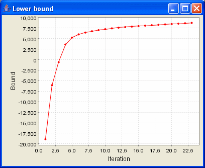
  During and after inference, the value of the lower bound will be displayed on this button. Clicking the button will cause a graph to appear, showing how the bound changes with each iteration of the algorithm. Here is an example of such a graph:

Data Views

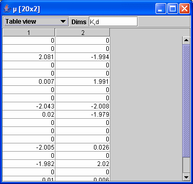
During and after inference, the expected value of each variable under the approximate posterior can be monitored using a data view. To see a data view for a node, simply double-click on the node. A window will pop up, like this one:

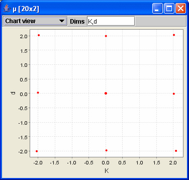
The title of the window contains the name and dimensionality of the node. The data will then be displayed in a table, Hinton diagram, image or chart view. You can change the view type using the drop-down list e.g. to a chart:

The text box labelled Dims shows the dimensions of the data being displayed. You can edit this list e.g. to transpose the display. The current views are limited to displaying 2D data - if you attempt to view data of higher dimensionality, an error message will be displayed. You can view a subset of such data by entering only some of the dimensions into the Dims box (the remaining indices will be set to zero).

Data views are intended to act as a helpful tool, not provide an exhaustive range of display options. If you want a different view, save the results to a Matlab file and use Matlab to display your results.